Investigating the Federal Reserve's Influence on the S&P 500
by Sam Funk

Overview
Being in Chicago, I found it fitting to investigate two of its most popular scholarly figures. The works of Eugene Fama and Milton Friedman had a profound impact on my schooling and economic proclivities. For this project, I wanted to devise a research question that would incorporate theories from both of these economists. Since regression would be involved, I decided to look into Fama’s Efficient Market Hypothesis, which states, in varying degrees, asset prices fully reflect all available information and are always at fair value. Even with sound historical data, Fama posits it is nearly impossible to consistently outperform the market as well as accurately predict future returns in the long run. As for Friedman, I always found his calls for the Federal Reserve to implement monetary policy rules highly interesting. He argued it was in the best interest of the American economy for the Fed to remain predictable as they try to reach their goal of price stability. These rules would tamp down uncertainty and increase the measurability of Fed activity and its accountability. Now, with these two concepts in mind, I want to test each simultaneously. I want to see if the Federal Reserve’s activities have any measurable effect on the American stock market and if this behavior is predictable. To do so, I will need to see how different daily Fed-related events impact the movements of the S&P 500.
Data
My initial plans for this project were quite ambitious. I wanted to scrape years of articles from multiple financial news sources, such as MarketWatch, Bloomberg, CNBC, Reuters, and the Financial Times. However, I soon realized that, although this could and can still be done, time was not on my side. Therefore, I decided to limit my data aspirations to one site over a four month period.
I scraped every article from MarketWatch from June through September 2017. This amounted to around 13,000 total articles. I took stock of each article’s subject and saved all the economic ones. Out of these, I distinguished whether the article was primarily focused on the Fed (strong cases) or if it simply mentioned a word such as ‘Yellen’ or ‘FOMC’ (weak cases). At this point, I had my data on the distribution of Fed articles against the rest of MarketWatch’s content.
My next source of data came from the Federal Reserve directly. I scraped the Fed’s calendar and took count of when specific events occurred. Some of these events included speeches, testimonies, FOMC meetings, and statistical releases. I also decided to include a variable that would try and measure the general public’s interest in the activity of the Fed. Using Google Trends, I pulled metrics on search terms like ‘unemployment’, ‘inflation’, ‘federal reserve’, and ‘yellen.’ I devised a weighted score that aimed to capture the daily levels and changes of interest in the Federal Reserve.
Finally, with the S&P 500 as my independent variable, I pulled historical, daily data for the GSPC (equivalent to the SPX index) from Yahoo Finance. The sources of all these data sets are listed below.
Exploratory Data Analysis
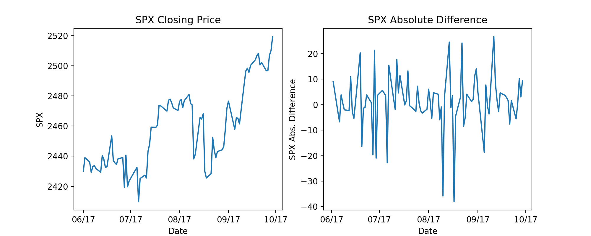
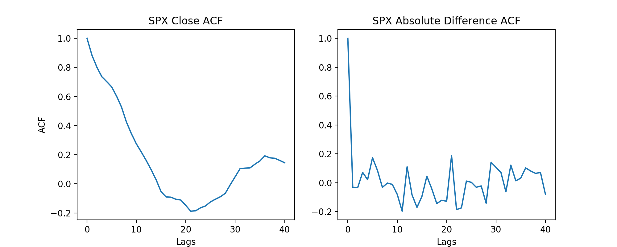
Before I jumped into any regressions, I needed to take a good look at my data. One issue I ran into immediately was the fact I was using stock market data, which is a sequence of discrete-time data. When it comes to linear regressions, time series data can prove to be problematic since individual data points can potentially be influenced by past or future data points. To solve this issue of autocorrelation, I took the daily difference of the SPX and used those values as my target variable. This technique of differencing greatly reduces autocorrelation and the underlying trend present in the closing SPX values as well as making the data stationary. At this point, I was able to make the assumption that my data would be able to be used for linear regression. It is important to note that my results could still potentially be affected by time, which could lead to spurious results.
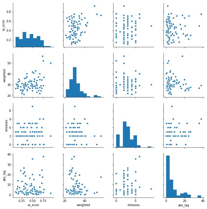
As for my features, I narrowed the relevant variables down to ‘Fed’ articles per, the proportion of ‘Fed’ articles to economic articles, daily statistical releases, and the weighted Google Trends score. These were the only variables with any semblance of correlation with the SPX. It should be noted that the first two features related to ‘Fed’ articles had a high positive correlation. The next section on my regression model will address this issue. Finally, I transformed the dependent variable by taking the absolute value of the daily difference in index level. This decision was made with the naive nature of my features in mind. None of the articles or Fed events were measured on the connotation of their content, therefore, making the index’s change in magnitude more important than the direction.
Regression Model
Since I used daily variables, my data set was shrunk down to only 84 observations (trading days from June-September 2017). Because of this fact, I was unable to divide my data into train and test sets. I was able to run a cross validated linear regression with Lasso regularization, which tries to further optimize the model’s parameters. The regularization was useful since I included two features that were positively correlated. My final independent variables included were the ‘Fed’ articles per day, statistical releases, and the weighted Google Trend score.
Results
The best model (alpha of 1e-5 with an intercept) did not perform well. It scored a mean squared error of 62.51 and an R-squared of 0.04, meaning the model does very little to explain the variability of the absolute daily change of the SPX. Additionally, none of the coefficients were statistically significant. Looking at the predictions and residual distribution, we can see this model violates multiple linear regression assumptions.
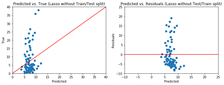
This failure in modeling could be attributed to the time series nature of the data, however, it is more likely the features included are simply not sufficient in predicting the movement of the SPX. Many other exogenous variables such as macroeconomic factors and corporate earnings would need to be incorporated into the model. On top of that, this model could be improved by increasing the time horizon and number of news sources used. Beyond that, a deeper analysis of the content of each relevant article using Natural Language Processing could lead to further insights into the Fed’s activity and its corresponding effects on the market. Although this model did not accurately explain what it was set out to do, it does reinforce Fama’s hypothesis that it is difficult to predict future returns and Friedman’s argument that the Federal Reserve should be calculated and credible.
The presentation can be found here.
Subscribe via RSS